Differential SystemToCell Signaling Across Conditions
Micha Sam Brickman Raredon
2022-07-20
05 Differential SystemToCell.RmdNICHES is also able to compare SystemToCell signaling across conditions to estimate changes in sensed-microenvironment due to altered experimental conditions or altered tissue state. To perform this operation, NICHES creates a measurement of ligand coming from the whole system by taking the mean of all sending cells for each ligand mechanism, and then multiplying this value with the cognate receptor mechanism expression on each receiving cell. The workflow has been designed this way so that altered cell compositions between samples will have a measurable effect on the NICHES output. This allows insight into the alterations to network connectivity which occur due to the development or elimination of celltypes in dynamic processes and can help users to identify cell-cell relationships of interest for further investigation.
However, it also means that care must be taken when setting up the computational workflow. In particular, we recommend that the number of cells analyzed in each condition be standardized, to avoid potential artifacts which might be caused by taking the mean in different conditions using different denominators.
We will demonstrate this workflow and functionality using the publicly available ‘ifnb’ dataset within SeuratData which allows comparision of IFNb-stimualted PBMCs versus control PBMCs.
Load Data and Explore Metadata
library(SeuratData)
#InstallData("ifnb")
data("ifnb")
table(ifnb@meta.data$stim,ifnb@meta.data$seurat_annotations)
#>
#>        CD14 Mono CD4 Naive T CD4 Memory T CD16 Mono    B CD8 T T activated   NK
#>   CTRL      2215         978          859       507  407   352         300  298
#>   STIM      2147        1526          903       537  571   462         333  321
#>
#>          DC B Activated   Mk  pDC Eryth
#>   CTRL  258         185  115   51    23
#>   STIM  214         203  121   81    32
This dataset contains two experimental conditions, annotated STIM and CTRL. As before, prior to running NICHES, we will split the dataset into two objects, one representing each experimental condition. This way, cells will only be crossed with cells in the same experimental condition. We also make sure that the data are normalized.
Split by Experimental Contion
# Normalize the data
ifnb <- NormalizeData(ifnb)
# Set idents so that celltypes are in active identity slot
Idents(ifnb) <- ifnb@meta.data["seurat_annotations"]
# Split object into STIM and CTRL conditions, to calculate NICHES objects separately
data.list <- SplitObject(ifnb, split.by="stim")
In contrast to the previous vignette, we are interested in the SystemToCell signaling output. Because of this, we advise standardizing the number of cells in each condition that are input into NICHES for each condition. This is one simple approach for how to do this:
# Define the maximum number that can be sampled from all conditions
max.cells <- min(ncol(data.list[[1]]),ncol(data.list[[2]]))
# Downsample to the same number of cells for each condition
for (i in 1:length(data.list)){
  Idents(data.list[[i]]) <- data.list[[i]]$stim
  data.list[[i]] <- subset(data.list[[i]],cells = WhichCells(data.list[[i]],downsample = max.cells))
  Idents(data.list[[i]]) <- data.list[[i]]$seurat_annotations
}
# Check resulting distributions and that the totals are the same
distribution <- data.frame(CTRL = table(Idents(data.list[[1]])),
                            STIM = table(Idents(data.list[[2]])))
distribution <- reshape2::melt(distribution)
ggplot(data = distribution,aes(x = STIM.Var1,y=value,fill = variable))+geom_bar(stat='identity',position='dodge')+
  theme(axis.text.x = element_text(angle = 45, vjust = 1, hjust=1))+
  ggtitle('Number of Cells Per Condition')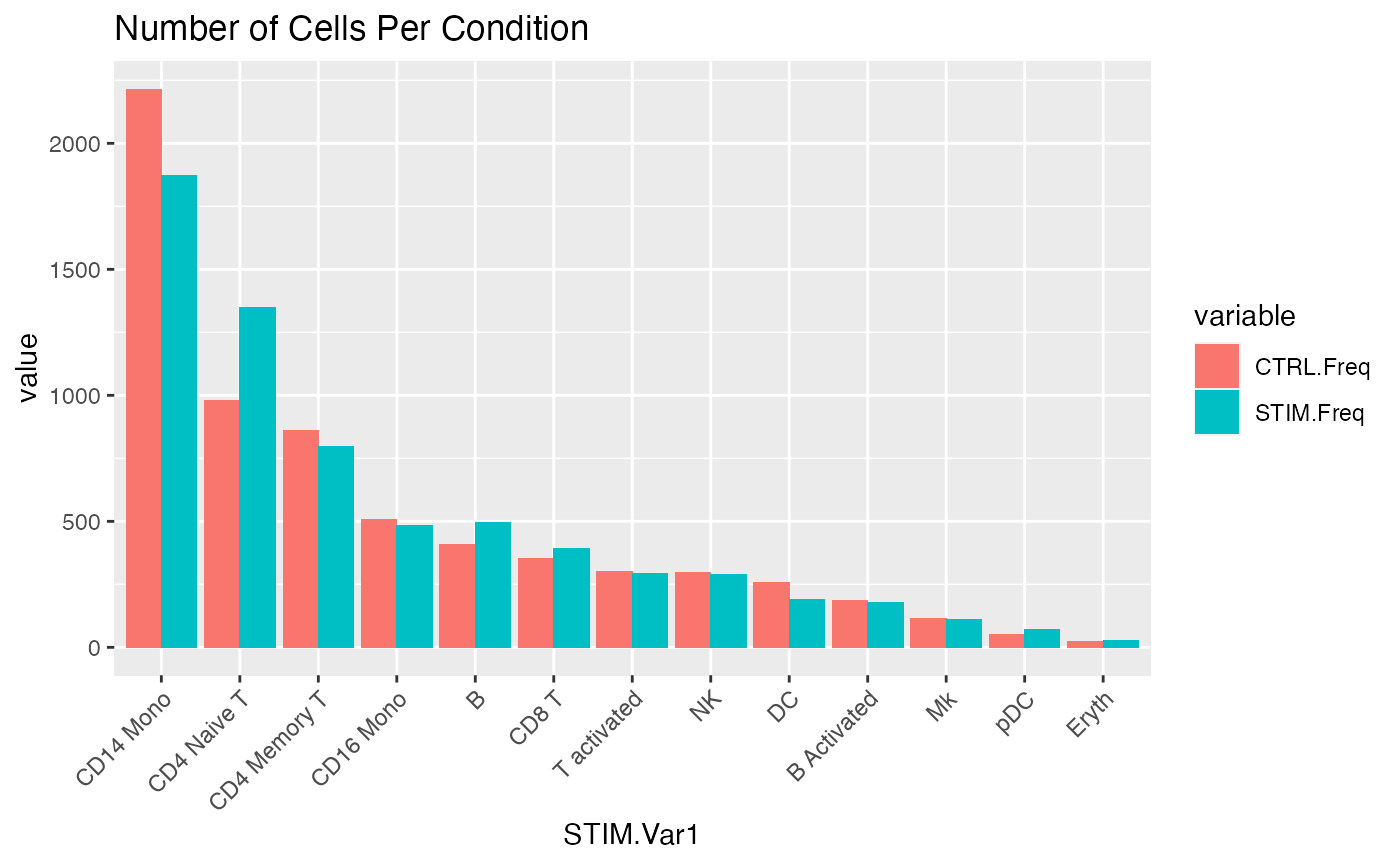
We now are prepared to calculate SystemToCell signaling for each experimental condition.
Run NICHES
# Run NICHES on each system and store/name the outputs
scc.list <- list()
for(i in 1:length(data.list)){
  print(i)
  scc.list[[i]] <- RunNICHES(data.list[[i]],
                             LR.database="fantom5",
                             species="human",
                             assay="RNA",
                             cell_types = 'seurat_annotations',
                             min.cells.per.ident=1,
                             min.cells.per.gene = 50,
                             meta.data.to.map = c('orig.ident','seurat_annotations','stim'),
                             SystemToCell = T,
                             CellToCell = T,
                             blend = 'mean')
}
#> [1] 1
#> [1] 2
names(scc.list) <- names(data.list)
NICHES provides output as a list of objects or tables, because it is capable of providing many different styles of output with a single run. Let’s isolate a specific output style we are interested in and tag it with appropriate metadata (redundant here, but good practice)
Isolate Output of Interest
temp.list <- list()
for(i in 1:length(scc.list)){
temp.list[[i]] <- scc.list[[i]]$SystemToCell # Isolate SystemToCell Signaling, which is all that will be covered in this vignette
temp.list[[i]]$Condition <- names(scc.list)[i] # Tag with metadata
}
We can then merge these NICHES outputs together to embed, cluster, and analyze them jointly:
Merge and Clean
# Merge together
scc.merge <- merge(temp.list[[1]],temp.list[2])

# Clean up low-information crosses (connectivity data can be very sparse)
VlnPlot(scc.merge,features = 'nFeature_SystemToCell',group.by = 'Condition',pt.size=0.1,log = T)
scc.sub <- subset(scc.merge,nFeature_SystemToCell > 5) # Requesting at least 5 distinct ligand-receptor interactions per measurementLet’s now perform an initial visualization of signaling between these two conditions, which we do as follows:
Visualize full dataset
# Perform initial visualization
scc.sub <- ScaleData(scc.sub)
scc.sub <- FindVariableFeatures(scc.sub,selection.method = "disp")
scc.sub <- RunPCA(scc.sub,npcs = 50)
ElbowPlot(scc.sub,ndim=50)
We choose to use the first 10 principle components for a first embedding:
scc.sub <- RunUMAP(scc.sub,dims = 1:10)
p1 <- DimPlot(scc.sub,group.by = 'Condition')
p2 <- DimPlot(scc.sub,group.by = 'ReceivingType')
plot_grid(p1,p2)
Predictably here, there is a big observed shift between conditions.
Focus on a single receiving cell of interest
unique(scc.sub@meta.data$ReceivingType)
#>  [1] "CD14 Mono"    "pDC"          "CD4 Memory T" "T activated"  "CD4 Naive T"
#>  [6] "CD8 T"        "Mk"           "B Activated"  "B"            "DC"
#> [11] "CD16 Mono"    "NK"           "Eryth"
# Define ReceivingType of interest
COI <- "DC"
# Loop over ReceivingType of interest, subsetting those interactions, finding markers associated with the comparison of interest (stimulus vs control) and  create a heatmap of top markers:
lapply(COI, function(x){

  #subset
  subs <- subset(scc.sub, subset = ReceivingType == x)

  #print number of cells per condition
  print(paste0(x , ":  CTRL:", sum(subs@meta.data$Condition == "CTRL")))
  print(paste0(x , ":  STIM:", sum(subs@meta.data$Condition == "STIM")))

  #set idents
  Idents(subs) <- subs@meta.data$Condition

  #scale the subsetted data
  FindVariableFeatures(subs,assay='SystemToCell',selection.method = "disp")
  ScaleData(subs, assay='SystemToCell')

  #find markers (here we use ROC)
  markers <- FindAllMarkers(subs, test.use = "roc",assay='SystemToCell',
                            min.pct = 0.1,logfc.threshold = 0.1,
                            return.thresh = 0.1,only.pos = T)

  #subset to top 10 markers per condition
  top10 <- markers %>% group_by(cluster) %>% top_n(n = 10, wt = myAUC)

  #Make a heatmap
  DoHeatmap(subs,group.by="ident",features=top10$gene, assay="SystemToCell") +  ggtitle("Top DE SystemToCell Mechanisms, CTRL vs STIM: ",x)

})
#> [1] "DC:  CTRL:258"
#> [1] "DC:  STIM:190"
#> [[1]]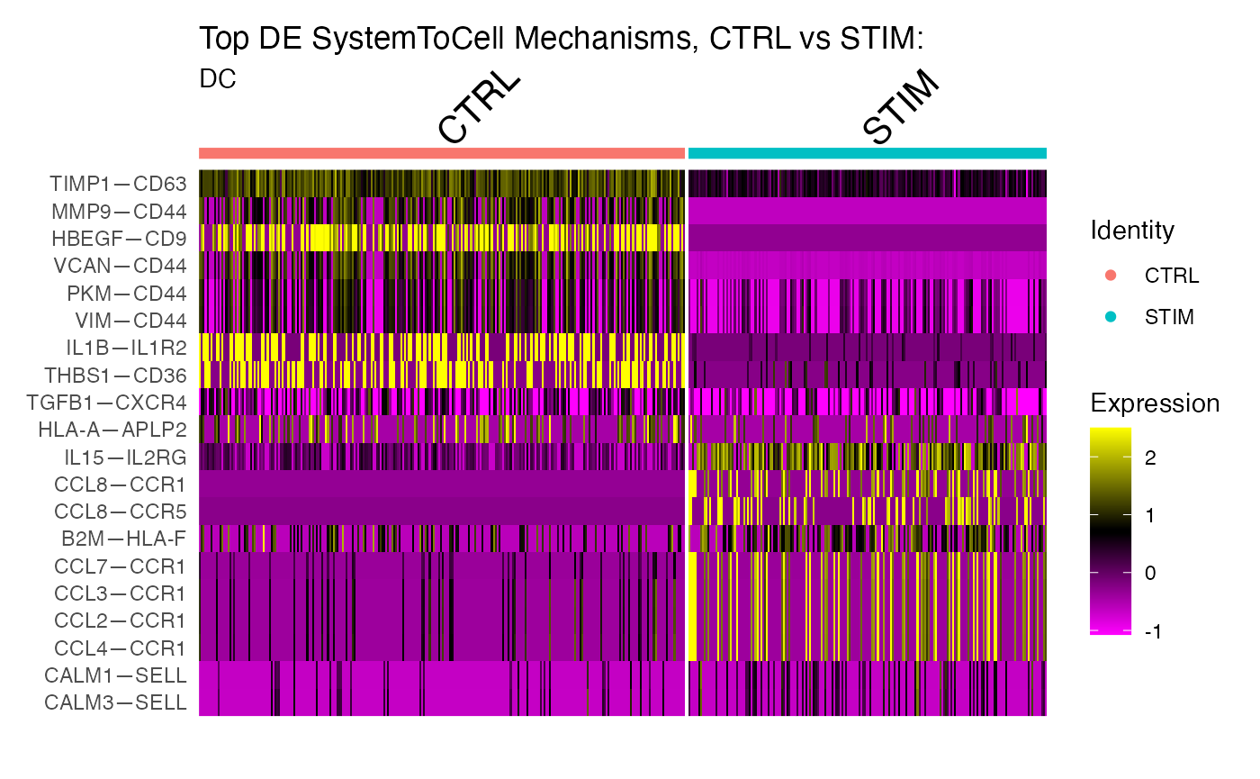
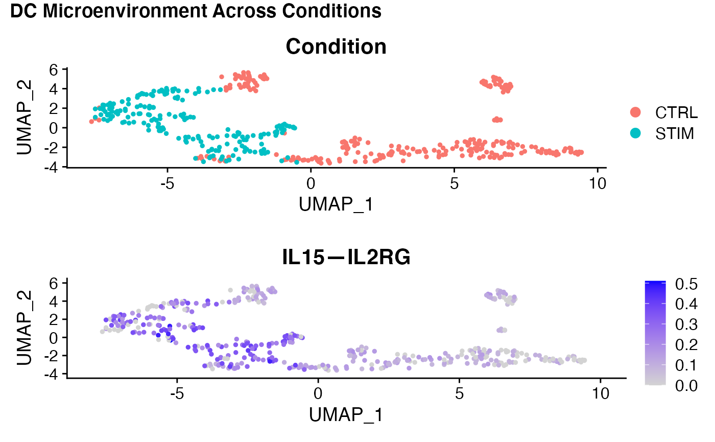
Some of these markers we have already identified in the previous vignette in whcih we queried the CD14 Mono—DC relationship. However, some of these mechanisms are new to us. IL15-IL2RG is new from this analysis. Let’s see where this signal is coming from in the original data, and if it is more likley an effect of altered ligand expressivity in the tissue or altered receptor expressivity on DCs:
p1 <- VlnPlot(ifnb,'IL15',split.by = 'stim',pt.size = 0,log=T)
p2 <- VlnPlot(ifnb,'IL2RG',split.by = 'stim',pt.size = 0,log=T)
plot_grid(p1,p2,ncol=1)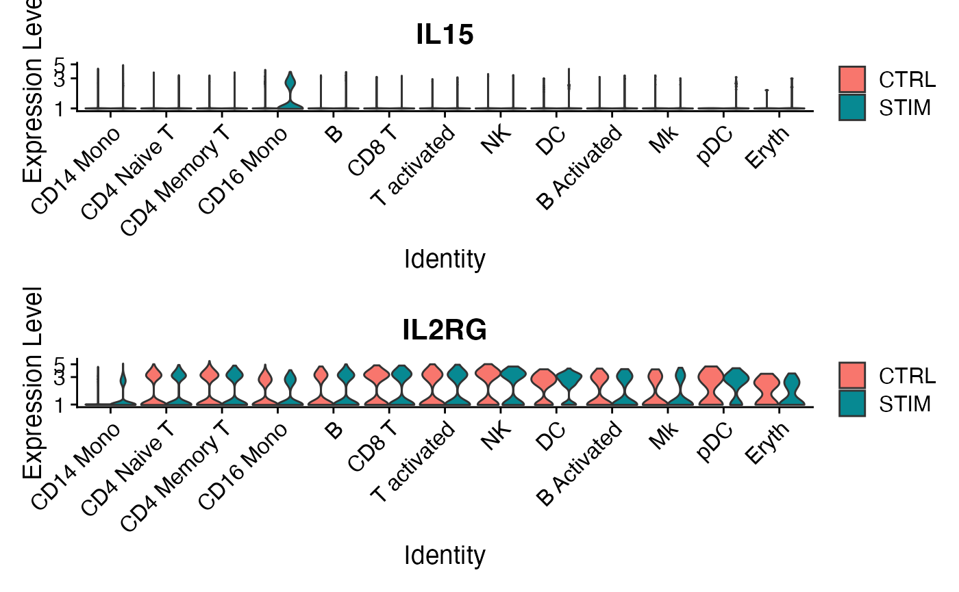
It looks like this pattern is most likley an effect of upregulated IL15 expressivity in the system by CD16 Mono cells. Let’s probe this further:
VlnPlot(scc.sub, 'IL15—IL2RG',split.by = 'Condition',pt.size = 0)
subs <- subset(scc.sub, idents = 'DC')
subs <- ScaleData(subs)
subs <- RunPCA(subs)
subs <- RunUMAP(subs,dims = 1:5)
p1 <- DimPlot(subs,group.by = 'Condition')
p2 <- FeaturePlot(subs,'IL15—IL2RG')
title <- ggdraw() +
  draw_label(
    "DC Microenvironment Across Conditions",
    fontface = 'bold',
    x = 0,
    hjust = 0
  ) +
  theme(
    # add margin on the left of the drawing canvas,
    # so title is aligned with left edge of first plot
    plot.margin = margin(0, 0, 0, 7)
  )
plot_grid(title,p1,p2,ncol=1,rel_heights = c(0.1, 1,1))